Behavioral Cloning

Josh Smith

---

Behavrioal Cloning Project

The goals / steps of this project are the following:

• Use the simulator to collect training and validation data
• Build, a convolution neural network in Keras that predicts steering angles from images
• Train and validate the model with a training and validation set
• Test that the model successfully drives around track one without leaving the road
• Summarize the results with a written report

Rubric Points

Here I will consider the rubric points individually and describe how I addressed each point in my implementation.

---

Files Submitted & Code Quality

1. Submission includes all required files and can be used to run the simulator in autonomous mode

My project includes the following files:

• model.py containing the script to create and train the model
• drive.py for driving the car in autonomous mode
• data_processing.py containing the scripts for data generation
• model.h5 containing a trained convolution neural network
• writeup_report.md or writeup_report.pdf summarizing the results

2. Submission includes functional code

Using the Udacity provided simulator and my drive.py file, the car can be driven autonomously around the track by executing

python drive.py model.h5

The model can be trained by executing the following.

python model.py --train_folder data/train/ --validation_folder data/validation/ --epochs 2 --batch_size 256

3. Submission code is usable and readable

The model.py file contains the code for training and saving the convolution neural network. The file shows the pipeline I used for training and validating the model, and it contains comments to explain how the code works.

The data_processing.py file contains the data processing pipeline and has comments to explain the process. I would like to explore the use of Keras lambda layers to streamline the preprocessing in the future.

Model Architecture and Training Strategy

1. An appropriate model architecture has been employed

My model consists of a convolutional neural network with 3 5x5 filters with stride 2 with a residual connection followed by 2 1x1, 3x3, 1x1 filter blocks with a residual connection. The residual blocks are followed by three fully connected layers. All layers used ReLU activation to introduce non-linearity. The output layer uses a tanh function to conveniently limit steering angles to +/- 1.

2. Attempts to reduce overfitting in the model

The convolutional layers are naturally resistant to overfitting and the fully connected layers were minimize to reduce the possibility of overfitting. To further combat overtraining early termination was used by monitoring the loss between the train and validation dataset. The validation set was generated and kept completely separate from the training set.

3. Model parameter tuning

The model is very sensitive to the hyperparameters and fastidious notes were required to find parameters that worked well. Using NVIDIA's DAVE-2 model allowed for the search of hyperparameters without also requiring the search of a suitable network. To obtain suitable results the following hyperparameters required tuning:

• Batch Size FLAG --batch_size
• Samples per Epoch model.py line 110
• Epochs FLAG --epochs
• Left/Right Image Steering Offset data_processing.py line 84
• Random Crop Steering Adjustment data_processing.py line 42

The model used an adam optimizer, so the learning rate was not tuned manually.

4. Appropriate training data

Training data was selected to show a combination of ideal driving and recovery driving. Data with low velocity was removed from the training set. The low-velocity data in many cases was poor driving behavior and would not be desirable to train on. Data with no steering input was not completely removed but only a random portion was allowed into the training set. This was done to normalize the dataset.

For details about how I created the training data, see the next section.

Model Architecture and Training Strategy

1. Solution Design Approach

To get off the ground running I first implemented NVIDIA's DAVE-2 architecture. Using the known, viable architecture as a starting point allowed me to develop the preprocessing pipeline and find suitable hyperparameters.

Finding a combination of hyperparameters that yielded suitable results turned out to be much more difficult than developing the architecture its self.

During training, I utilized only the left and right camera images. For each image, a steering offset was applied to the actual steering value. The thought here was that the left image would appear like the car had drifted to the left and required right steering input to move back to the center. This effectively doubled the training set as well as amplified the steering commands to include larger corrections that would not normally be seen during data capture. Originally I included the center image in the dataset but was unable to get consistent results. I expect that including the center image narrows the acceptable range for the steering offset hyperparameter.

Here is an example of the three camera images with the applied steering offset:

To manage a large number of images the Keras fit_generator function was utilized along with the batch_generator function in data_processing.py. This would randomly draw a sample batch from the cleaned dataset, preprocess and deliver to the fit_generator.

To determine a good epoch count (and the number of samples per epoch) I would monitor the loss of the train data and validation data. If the validation loss stopped decreasing and the training loss is continuing to decrease this was an indicator that the model is overfitting. The epoch count was reduced to minimize the overfit. In most cases, the model was trained in one or two epochs consisting of 20,000 samples.

After the data processing pipeline was established I started looking at improving the DAVE-2 architecture. I tried adding more convolutional layers, increasing filter count, adding residual connections, using dropout on increased fully connected layers, changing the activation of the hidden layers to Exponential Linear Units, using Leaky ReLU. In the end, the DAVE-2 architecture is, unsurprisingly, very good and would require some time to significantly improve.

After training the model was always evaluated in the simulator to determine not only how well the model stayed on the road but also to determine how smoothly the model drove. Overfit models tended to oscillate in the road sections that had low curvature.

I found that this problem, in general, was very prone to overfitting. The normal tactics of applying dropout, regularization and early termination all seems to produce unstable driving patterns on larger architectures. Simple model architectures produced much smoother driving characteristics than complex models with overfitting techniques applied.

2. Final Model Architecture

model.py line 56

The final model used a residual connection between each convolutional block. ReLU activation was used after the residual merge.

The first residual block contains a 5x5 convolution with 'same' padding with a stride of 2 to reduce dimensionality. The dimensionality reduction was matched in the residual connection by using a 1x1 convolution with a stride of 2. This first block was repeated three times with filter sizes of 24, 36 and 48.

The second residual block contains a 1x1, 3x3 and 1x1 bottleneck configuration where the first 1x1 and 3x3 convolution reduced filter count by a factor of 4 and the last 1x1 expanded the filter count back. Rather than using this to reduce computational cost, it was used to reduce overfitting and smooth the driving behavior. This block was repeated twice with an expanded filter size of 64.

This was followed by a block of fully connected layers using ReLU activation of sizes 100, 50 and 10. No dropout was employed and overfitting was again reduced by keeping model order low.

The output uses a tanh activation.

The model uses a mean squared error loss function with the adam optimizer.

3. Creation of the Training Set & Training Process

Data Collection

Several laps in each direction on the track were recorded where I attempted to stay centered in the lane. Here is an example image of center lane driving:

With only center lane driving there would be no examples of what should be done if the car happens to get slightly off line. This recovery behavior was recorded by driving several laps in each direction drifting to one edge of the track, turning recording on and correcting back to centerline. The recording was turned off when drifting to the edge as to not encourage the model to repeat this behavior. Here is an example of the start of a recovery position:

This resulted in a total training set size of 21,801 data points.

The validation set was constructed by completing several laps around the track driving safely resulting in 4,727 data points. This set was used exclusively for validation.

Data Augmentation

Data augmentation was used to improve generalization and was applied to the batch.

Applying a random shadow

data_processing.py (line 7) A random shadow was applied to the general road area of the image by overlaying a random black triangle with random opacity.

Applying a random crop

data_processing.py (line 36) A random crop was applied to the image which cropped the original 320x160 image to 200x68. The crop position was limited to +/- 20 pixels vertically but could span the whole horizontal range. Since the horizontal offset of the crop simulates the car being slightly offset from the actual position the steering angle was adjusted based on a linear factor applied to the magnitude of the horizontal offset from center.

Applying a random horizontal flip

data_processing.py (line 24) A random flip was applied to the images with a corresponding flip to the sign of the steering angle. This was done to reduce the bias towards a given steering direction.

Normalization

Images were normalized using a contrast normalization with cutoff followed by a histogram equalization then the range was rescaled to be +/- 1.

Simulation Results

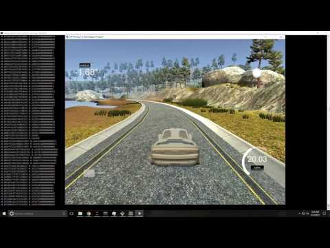
Using the final network described above the model was trained for 2 epochs of 20,000 samples with a batch size of 256. The results of the model produced very smooth driving characteristics that were able to drive safely for hours. Here is an example run from this model: